The Bellman Optimality Equation and Markov Decision Processes in Reinforcement Learning

AI’s capabilities are fundamentally driven by massive computational power. 

Computation acts as the “engine” that allows AI systems to function. Modern AI models — especially deep learning networks and large language models, demand immense processing capacity to perform the millions (or even billions) of mathematical operations involved in training and inference.

However, AI’s effectiveness doesn’t rely on computation alone. Its full potential stems from the synergy between large-scale compute, high-quality data, and advanced learning algorithms — 3 distinct but interdependent components that rely on one another.

Compute provides the raw processing power to train and deploy models. Data forms the foundation for pattern recognition and learning. And algorithms determine how the system interprets that data, learns from it, and delivers accurate, reliable outputs.

In this post we will be discussing how an optimality condition called the Bellman equation, that is the foundation for many key algorithms for solving what are called Markov Decision Processes, gives AI agents the ability to navigate uncertainty through methodical decision-making.

To start off, RL is the branch of AI that allows machines to make decisions, adapt, and correspondingly display goal-directed behaviour. This is done through the use of giving rewards to an AI agent: a key decision-maker whose goal is to reap as much of these rewards as possible, which are given only when they align more and more with your goals.

At the hub of this ability amongst other things, stand the Bellman equation and the Markov Decision Process (MDP) — the mathematical pillars that underpin the majority of theoretical RL. These frameworks allow machines to interpret experience, and refine their behaviour through continual learning. For this reason is that I begin here: without MDPs and the Bellman optimality equation, modern reinforcement learning would lack the very foundations of its goal-directed behaviour. Of course, not all RL methods rely on MDPs and Bellman equations directly — some instead learn from reward signals only, or treat actions as trial and error without modeling state transitions. We will get into all this later.

A side note before we continue: for this first post, we will focus on the elementary and conceptual foundations of these topics. In later entries, I will then expand into the quantitative and more elaborate details.

Now, imagine that you’re leaving work and trying to decide how to get home. Do you take the highway, which is usually fast but prone to traffic jams, or the back roads, which are slower but reliable?

This is the kind of puzzle we face repeatedly: How do I make the best decision now, knowing it will affect what happens next?

The Bellman Optimality equation:

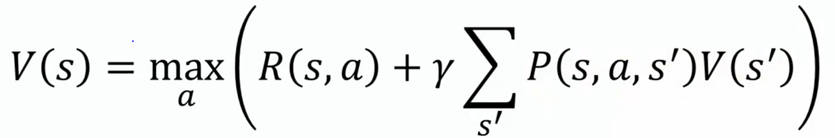
In artificial intelligence, this almost universal question is captured by a beautiful piece of math: the Bellman Optimality equation, not to be confused with the Bellman expectation equation (will be discussed later).

The former, is the compass that tells machines (and, indirectly, us) how to choose not just for immediate reward, but for long-term success as well.

We see this because it includes the max over actions, which encodes the principle of choosing the best possible action at every step. It calculates the value of states assuming the agent acts optimally. Within the context of self-driving cars for example, states can be an intersection, a railroad crossing, or a parking lot. The specific form the state takes is entirely up to the engineer or designer of the RL problem, given it provides all the information relevant to the agent for making decisions.

This equation is the hidden engine behind AlphaGo’s ultimate victory over world champions, OpenAI’s bots that mastered the strategy game Dota 2, and even the decision-making logic in self-driving cars.

All things considered, this Bellman equation cannot stand alone; it relies on the Markov Decision Process (MDP) framework, which defines the states, actions, transitions, and rewards. Without an MDP providing this structure, the Bellman equation has no problem to solve in order to reach long-term success.

To formally reach a definition: A Markov Decision Process (MDP) defines states, actions, rewards, and transition dynamics under uncertainty, giving the Bellman optimality equation the structure it needs to express the best possible long-term value of each state.

Although beyond our current scope, not all algorithms use the Bellman equation or the MDP in the same way; the distinction depends on whether the method is model-based or model-free, with the ‘model’ referring to the agent’s internal representation of the environment.

Just to briefly explain: model-based reinforcement learning would be like planning your actions by understanding the rules of a game, while model-free learns by trying things out and seeing what works.

The MDP: Taking the Highway or Backroads?

The details that an MDP gives us are in this sequence/tuple, (S, A, P, R, y):

• States (S): Where you are right now. For example: “at the office,” “on the highway,” “stuck in traffic,” or “driving on back roads.”
• Actions (A): The choices you can make. For example: “take highway” or “take back roads.”
• Transition probabilities (P): The likelihood of moving from one state to another, given your action. For instance, taking the highway might give you an 80% chance of smooth driving but a 20% chance of hitting a jam.
• Rewards (R): The payoff you receive. A shorter commute time is a higher reward, while getting stuck in traffic is a penalty.
• Discount Factor (γ): Represented by the Greek letter gamma, the discount factor will be a value between 0 and 1 that balances the importance of immediate rewards versus long term rewards. When closer to 0, the agent will choose short term rewards, and when closer to 1, it will be farseeing and will prioritize better long term outcomes.

The Markov Property and Markov Chains

Much like working memory in the human mind, the Markov property ensures that the present state embodies all the information needed to make the next decision. By design, this spares an agent from the weight of all past experiences, enabling it to capture the independence, and accordingly plan with clarity and efficiency in the moment. The Bellman equation then operationalizes it, enabling the AI agent to weigh the expected utility of each choice recursively, refining the choices by balancing the value of immediate outcomes against the promise of future rewards. The Markov property is what allows us to define an MDP at all. It ensures that states are self-contained snapshots of everything relevant for decision-making.

This principle naturally leads to the concept of a Markov chain. A Markov chain is a sequence of states linked by transition probabilities, where the next state depends solely on the current one. Specifically, it is a mathematical model of stochastic processes — a way of describing how a system moves between states with certain probabilities. It essentially asks, "Given where you are right now, what is the probability of ending up in each possible next state?"

As an example, imagine again that you are leaving work and deciding how to get home. Your current “state” might be standing at the office parking lot. From there, you might take the highway or the backroads. Each of these choices corresponds to a new state, and each carries a probability of leading to another state — perhaps the highway is usually fast but has a 40% chance of gridlock, while the backroads are slower but have a much higher chance of steady progress.

Wrapping it up, while the Markov property ensures that only your current location matters when determining what comes next. The Markov chain is the actual process that unfolds as you move from state to state under those probabilities.

Partially Observable Markov Decision Processes (POMDPs)

In practice, however, most environments are not so neatly defined. Agents often operate under uncertainty, with only partial glimpses of the world. This is where Partially Observable Markov Decision Processes (POMDPs) come in. The POMDP framework provides the theoretical machinery to formalize and solve decision problems where incomplete information is the rule, not the exception.

Unlike standard MDPs, where the agent knows its exact state, a POMDP assumes the agent only receives fragments of information — observations that are noisy or incomplete — and must infer what is really happening. Take our backroads example: in the fully observable case, you know precisely whether traffic is clear or jammed and can decide accordingly. But in some cases, you may only glimpse a few cars ahead or receive outdated traffic reports; you never see the entire road. You must act based on partial clues, updating your “belief” about conditions as you go.

This distinction matters greatly because most real-world problems resemble POMDPs, not MDPs.

This first post has set up the stage by introducing some of the core ideas. In the next ones, I will integrate the mathematics that is fundamental to them. I will also expand into topics such as the Markov property, rewards and returns, the balance between exploration and exploitation, and the role of policies (π) in guiding decisions.

Thanks for reading, see you all next time.